3: Static Structural Analysis

With all the model setup out of the way, a static structural analysis system can be added. There are lots of other types of analyses, but for the solar car team this is what we typically analyze our parts with, This analysis requires the model not be in motion, i.e. all 6 degrees of freedom are somehow fixed between the included boundary conditions. If this is not true, the model will produce erroneous results.

SYSTEM CREATION

 For projects that plan on becoming very large, it is advisable to add this as its own system in the workbench project schematic. For smaller projects with only 1 or 2 load cases, it is fine to just add them within your mechanical model, which will turn the mechanical model into an analysis system. This can be done at the top of the home tab.

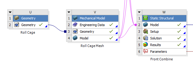
Fig 1. Adding and linking a static structural analysis system in workbench, good for large projects

--- OR ---

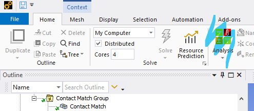
Fig 2. Adding an analysis system within mechanical model, good for small projects

Regardless, the model portion should start with a green checkmark, as that was completed in the previous guide. The only thing that needs user input for this analysis is the setup. By hitting the solve button, the solution will be generated, and then as long as the user has scoped result plots, the results will appear.

SETUP

A finite element analysis (FEA) needs boundary conditions (BCs) to function. These come in many varieties, for a structural analysis, typically in forces and displacements. FEA simply relates the forces in the model to the displacements of the nodes in the model through the model's stiffness. By giving it BCs, it can find all of the displacements and forces within the nodes of the model. From the displacement, strain (the derivative of displacement) and therefore stress can be found.

$k\begin{bmatrix}2 & -1 & -1 & 0 & 0 \\-1 & 3 & -1 & -1 & 0 \\ -1 & -1 & 3 & -1 & 0 \\ 0 & -1 & -1 & 3 & -1 \\ 0 & 0 & 0 & -1 & 1 \end{bmatrix}\begin{Bmatrix}0\\u_2\\u_3\\u_4\\0\end{Bmatrix}=\begin{Bmatrix}R_1\\F_2\\F_3\\F_4\\R_5\end{Bmatrix}$

Fig 3. A simple 1D finite element 5 node bar model matrix, from left to right: stiffness, displacement, force. BCs of 0 displacement on node 1 and 5 are applied

To start, right click on the study and hover over insert. This will pull up a large number of BCs. Most commonly you will use those highlighted in blue (force and fixed support). For more advanced control, those highlighted in pink (remote force and remote displacement) are preferred. However, they actually do the same thing, the second set just gives the user more control over the nodal behavior and degrees of freedom.

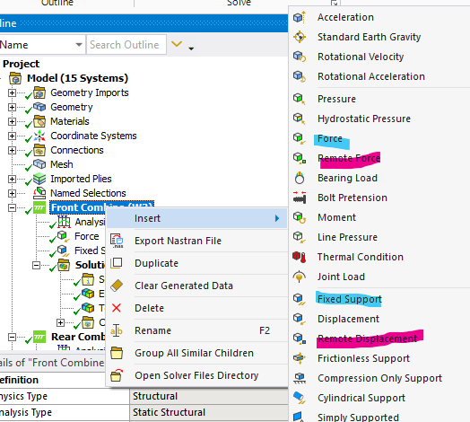
Fig 4. A screenshot of some BCs

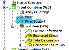
Next is result plots. Right click on solution and hover over insert to pull up a list of options. The most common plots utilized are equivalent stress and total deformation.

Analysis Settings

This contains some advanced controls such as what is saved by the solver and how the solver behaves. This may be necessary to modify if advanced result plot such as nodal force, nodal moments, and other plots are desired.