
Basics: 1D Bar Formulation
When solving for the various items of interest using the finite element method (FEM) such as displacement, stress, and strain, it is important to understand the basics of what is happening when you start pressing the various mesh, boundary condition, and solve buttons. In software, these perform very complicated versions of the basics tasks outlined below. Understanding exactly what is happening in each equation and each step is not necessarily super important, as you'll learn the specifics in the FEA class, but this will teach you more about what nodes and elements are.
At the most basic level, the FEM discretizes something into a set of nodes which form elements. The simplest form is a bar element, which represents a 1 dimensional spring with a node at either end and an element between the nodes with stiffness k. This stiffness can be a spring constant k, or if the model represents a real object such as a square bar , k can be calculated from the objects material properties and geometry.
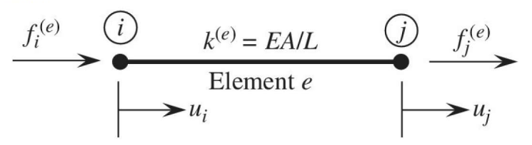
Fig 1. Example bar element
With this model, we can develop a relationship between the forces f and displacements u of the nodes, connected by the element from Hooke's law, which relates spring force to displacement by the spring constant k.
| $f_i=k(u_i-u_j)$ | (1) | |
| $f_j=k(-u_i+u_j)$ | (2) |
These can then be put into a matrix form by pulling out the common k terms and multiplying the displacement terms by an equivalent matrix. Review a numerical methods or linear algebra textbook for a deeper explanation of how matrix math works. This is the common way to represent finite element problems.
| $k\begin{bmatrix}1 & -1 \\-1 & 1\end{bmatrix}\begin{Bmatrix}u_i\\u_j\end{Bmatrix}=\begin{Bmatrix}f_i\\f_j\end{Bmatrix}$ | (3) |
Now this 1D problem can expanded with many nodes and elements chained together, as seen in figure 2. Each local set of nodes with an element between the two has the exact same matrix equation as equation 3. They can each be assembled together into a global matrix, which represents the whole system, where the subscript denotes the nodes and the superscript denotes the elements.
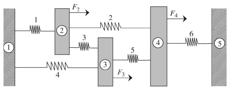
Fig 2. A large system of nodes and elements chained together, with applied forces (2,3,4) and fixed boundaries (1,5)
|
$k\begin{bmatrix}1+1 & -1 & -1 & 0 & 0 \\-1 & 1+1+1 & -1 & -1 & 0 \\ -1 & -1 & 1+1+1 & -1 & 0 \\ 0 & -1 & -1 & 1+1+1 & -1 \\ 0 & 0 & 0 & -1 & 1 \end{bmatrix}\begin{Bmatrix}u_1\\u_2\\u_3\\u_4\\u_5\end{Bmatrix}=\begin{Bmatrix}f_1^{(1)}+f_1^{(4)}\\f_2^{(1)}+f_2^{(2)}+f_2^{(3)}\\f_3^{(3)}+f_3^{(4)}+f_3^{(5)}\\f_4^{(2)}+f_4^{(5)}+f_4^{(6)}\\f_5^{(6)}\end{Bmatrix}$ |
(4) | |
|
$k\begin{bmatrix}2 & -1 & -1 & 0 & 0 \\-1 & 3 & -1 & -1 & 0 \\ -1 & -1 & 3 & -1 & 0 \\ 0 & -1 & -1 & 3 & -1 \\ 0 & 0 & 0 & -1 & 1 \end{bmatrix}\begin{Bmatrix}0\\u_2\\u_3\\u_4\\0\end{Bmatrix}=\begin{Bmatrix}R_1\\F_2\\F_3\\F_4\\R_5\end{Bmatrix}$ |
(5) |
The solution of this becomes fairly simply from the point of equation 5. when the applied forces of 2, 3, and 4 are known and the displacements of 1 and 5 are known to be zero (denoted by the cross hatching), each equation can be read across the rows and solved as a system of equations for the displacements of nodes 2, 3, and 4, and the reactions forces at nodes 1 and 5. This is known as the direct stiffness method.
While this is the simplest type of FEM problem, the use case can be extrapolated to deal with much more complex problems with advanced concepts. In your FEA class, you will start by tackling these 1 dimensional bar problems. More advanced concepts include beams and frames, although new methods using shape equations must be introduced to deal with solving the problems. At the highest level are 2D and 3D elements, which is what is utilized for practical FEA applications on the parts we design.
No comments to display
No comments to display